JMetalPy: An evolutionary algorithm framework for solving the optimization problems
Author: Yongfeng Gu, Date: May, 2020
0. Basic Introduction
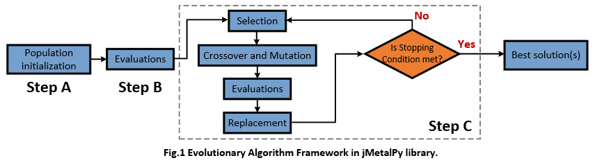
jMetalPy is a very nice toolkit providing commonly-used Evolutionary Algorithms (EAs) to solve the multi-objective or single-objective optimization problems. By using jMetalPy, one can easily implement the Greedy Search, Simulated Annealing, NSGA-II, IBEA, and SPEA2 algorithms for your own optimization problems. To give an intuitive impression of Evolutionary algorithm, I concluded a brief algorithm framework in jMetalPy is as follows (Step A, B, and C).
Technically, jMetalPy is a Python version of the jMetal framework, it's widely used and already integrated into the PYPI (which means you can easily install jMetalPy by typing command like pip install jmetalpy). Here are some related documentations,
- Pypi: https://pypi.org/project/jmetalpy/
- Homepage: https://jmetal.github.io/jMetalPy/index.html
- Github: https://github.com/jMetal/jMetalPy
- Documentation (out-of-date): https://readthedocs.org/projects/jmetalpy/downloads/pdf/stable/
- Publication: https://arxiv.org/pdf/1903.02915.pdf
However, the current documentation or tutorial online are either under construction or out of date, there seems to be no complete tutorial about the jMetalPy which makes it hard for beginners (like me) to master this toolkit. This is the main reason why I write this brief daily blog.
1. Single-objective Optimization
1.1 Problem
Knapsack Problem: The Knapsack Problem [1] is a problem in combinatorial optimization: Suppose that we have $n$ items, each with a weight ($w_i$) and a value ($v_i$), we try to select a subset ($T \subsetneqq \{0,1,2...,n\}$) of this items so that the total weight is less than or equal to a given limit ($W > 0$) and the total value is as large as possible.
$$ \mbox{Knapsack:} \ \ \ maximize \ \sum_{i \in T}v_i \ \ \ s.t., \sum_{i \in T}w_i \leq W $$To make problem easier to understand, we set $m=5$, $w = \{2,2,6,5,4\}$, $v = \{6,3,5,4,6\}$, and $W=10$.
Genetic Algorithm: The Genetic Algorithm [2] is a search heuristic that is inspired by Charles Darwin's theory of natural evolution. This algorithm reflects the process of natural selection where the fittest individuals are selected for reproduction in order to produce offspring of the next generation
[1] Liu. "Using Dynamic Programming to Solve the Knapsack Problem." Online Access.
[2] Tutorialspoint Team. "Introduction to Genetic Algorithm." Online Access.
1.2 Implementation
STEP-1: We first define the problem (Knapsack) we want to solve and the algorithm (GeneticAlgorithm) we expect to use. In this step, we need to set the basic hyper-parameters includes crossover and mutation operators, population size, and termination criterion.
:) The Knapsack problem is already defined in the jMetalPy library, we only need to call it.
from jmetal.problem.singleobjective.knapsack import Knapsack
from jmetal.algorithm.singleobjective import GeneticAlgorithm
from jmetal.util.termination_criterion import StoppingByEvaluations
from jmetal.operator import SPXCrossover, BitFlipMutation
from jmetal.operator.selection import RouletteWheelSelection, BinaryTournamentSelection, BestSolutionSelection

kp_problem = Knapsack(  # define the Knapsack problem
    number_of_items = 5,
    capacity = 10,
    weights = [2,2,6,5,4],
    profits = [6,3,5,4,6],
)

algorithm = GeneticAlgorithm(  # initialize the algorithm
    problem = kp_problem,
    population_size = 20,
    offspring_population_size = 20,
    mutation = BitFlipMutation(probability=1/kp_problem.number_of_variables),
    crossover = SPXCrossover(probability=0.8),
    selection = BestSolutionSelection(),
    termination_criterion = StoppingByEvaluations(max_evaluations=500)
)
STEP-2: We run our algorithm algorithm and get the result.
from jmetal.util.solution import get_non_dominated_solutions
from jmetal.lab.visualization import Plot

# run and get results
algorithm.run()
solution = algorithm.get_result()
print('Solution:',solution.variables, 'Maximum value:',solution.objectives[0])
:) Actually, people tend to use the Dynamic Programming algorithm to solve the 0/1 Knapsack Problem. Here I also provide a simple example of the Dynamic Programming algorithm. The maximum value is 15, which is consistent with the result of the Genetic Algorithm.
def solve_knapsack(num_items, weights, profits, W):
    '''
    solve the Knapsack problem using the dynamic programming algorithm
    ------------------
    :num_items : number of items
    :weights   : weight list for all items
    :profits   : value list for all items
    :W         : weight limit
    '''
    weights.insert(0,0)
    profits.insert(0,0)
    # construct table
    table = [[0 for j in range(W+1)] for i in range(num_items+1)]

    for i in range(1, num_items+1):
        for j in range(1, W+1):
            if weights[i] > j:
                table[i][j] = table[i-1][j]
            else:
                table[i][j] = max(table[i-1][j], (table[i-1][j-weights[i]] + profits[i]))

    return table[num_items][W]

solution = solve_knapsack(5, [2,2,6,5,4], [6,3,5,4,6], 10)
print('Maximum value:', solution)
2. Multi-objective Optimization
2.1 Problem
ZDT1 Problem: ZDT1 is a typical optimization problem from paper [1] and also a suitable example for introducing jMetalPy. Suppose that we have $m$ decision variables ($x_i$) to minimize two objective functions, i.e., $f_1$ and $f_2$. Each of $x_i$ should be in the range of [0,1]. ZDT1 problem can be summarized as follows,
$$ \mbox{ZDT1:} \ \ \begin{cases} minimize \ f_1 = x_1 \\ minimize \ f_2 = 1-\sqrt{f_1/g}, \ \ \ g = 1+\frac{9}{(m-1)}\sum_{i=2}^mx_i \end{cases} \ \ \ s.t., \ 0 \leq x_i \leq 1 $$NSGA-II Algorithm: NSGA-II is a famous multi-objective optimization algorithm introduced by [2]. In each selection, NSGA-II updates the population with a fast non-dominate sorting algorithm and crowding distance selection strategy.
[1]: E. Zitzler, K. Deb, and L. Thiele. "Comparison of Multiobjective Evolutionary Algorithms: Empirical Results". IEEE Transactions on Evolutionary Computation 8(2):173 - 195, 2000. [2]: K. Deb, A. Pratap, S. Agarwal, and T. Meyarivan. "A fast and elitist multiobjective genetic algorithm: NSGA-II". IEEE Transactions on Evolutionary Computation 6(2):182 - 197, 2002
2.2 Implementation
STEP-1: We first define the problem (ZDT1) we want to solve and the algorithm (NSGAII) we expect to use. In this step, we need to set the basic hyper-parameters includes crossover and mutation operators, population size, and termination criterion.
:) NSGA-II has its own default selection mode, we no longer redefine it in the program.
from jmetal.algorithm.multiobjective import NSGAII
from jmetal.operator import SBXCrossover, PolynomialMutation, BinaryTournamentSelection
from jmetal.problem import ZDT1
from jmetal.util.termination_criterion import StoppingByEvaluations

zdt1_problem = ZDT1()  # define the ZDT1 problem

algorithm = NSGAII(  # initialize the algorithm
    problem = zdt1_problem,
    population_size = 100,
    offspring_population_size = 100,
    mutation = PolynomialMutation(probability=1.0/zdt1_problem.number_of_variables, distribution_index=20),
    crossover = SBXCrossover(probability=0.8, distribution_index=20),
    termination_criterion = StoppingByEvaluations(max_evaluations=10000)
)
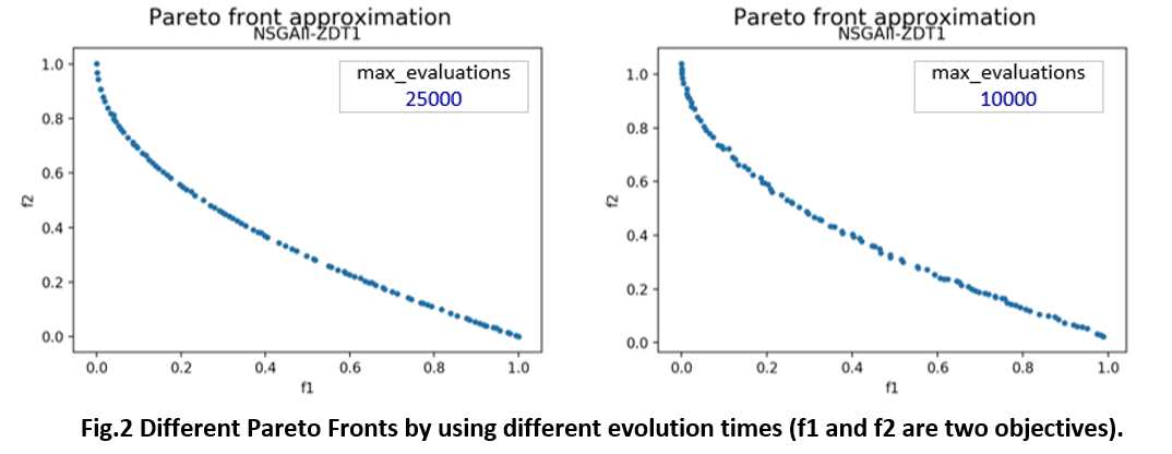
STEP-2: We run our algorithm algorithm and plot the Pareto Front on the graph. jMetalPy has its own plot interface jmetal.lab.visualization.Plot().
from jmetal.util.solution import get_non_dominated_solutions
from jmetal.lab.visualization import Plot

# run and get results
algorithm.run()
front = get_non_dominated_solutions(algorithm.get_result())

# plot the results
plot_front = Plot(title='Pareto front approximation', axis_labels=['f1', 'f2'])
plot_front.plot(front, label='\nNSGAII-ZDT1', filename='NSGAII-ZDT1', format='png')
3. Build Our Own Problem
In previous examples, we directly use the pre-defined optimization problem Knapsack and ZDT1. However, in practice, we have to build our own optimization problem to meet the specific requirements. Let's declare a new problem in just THREE steps!
STEP-1: Declare the customized problem class MyProblem and make it inherit one specific of the optimization problem (e.g., FloatProblem).
STEP-2: Initialize necessary parameters, such as number_of_variable, number_of_objectives, of the problem in the constructor (i.e., __init__).
STEP-3: Rewrite the functions evaluate() to define the way to evaluate the fitness score of each solution. This function takes the solution as the input and add the calculated fitness (i.e., objective attribute) to the solution.
Based on the above three steps, we re-build the ZDT1 problem in our own Python snippet,
from jmetal.core.problem import FloatProblem
from jmetal.core.solution import FloatSolution
import numpy as np

class MyProblem(FloatProblem):

    def __init__(self, number_of_variables = 30):
        super().__init__()

        # initial parameters
        self.number_of_variables = number_of_variables # decision variables
        self.number_of_objectives = 2
        self.number_of_constraints = 0
        self.lower_bound = [0.0 for _ in range(number_of_variables)]
        self.upper_bound = [1.0 for _ in range(number_of_variables)]

        self.obj_directions = [self.MINIMIZE, self.MINIMIZE] # both objectives should be minimized
        self.obj_labels = ['x', 'y'] # objectives' name

    def evaluate(self, solution) -> FloatSolution:
        '''
        define the way to evaluate one solution, i.e., calculate the objectives of each solution
        '''
        f1 = self.eval_f1(solution) # calculate the 1st objective
        f2 = self.eval_f2(solution, f1) # calculate the 2nd objective
        solution.objectives[0] = f1
        solution.objectives[1] = f2

        return solution

    def eval_f1(self, solution) -> float:
        return solution.variables[0]

    def eval_f2(self, solution, f1) -> float:
        g = sum(solution.variables) - solution.variables[0]
        constant = 9.0 / (solution.number_of_variables - 1)
        g = 1.0 + g*constant

        return 1.0 - np.sqrt(f1/g)

    def get_name(self):
        return 'My_ZDT1_problem'
In the above code snippet, there are few key points,
We achieved a inherit chain when building class
myProblem, i.e.,myProblem->FloatProblem->Problem, which means the solution type to our problem is the Float Solution.FloatProblemis defined in the file jmetal.core.problem.py, we can find the other types of problems, such asBinrayProblem,DoubleProblemandPermutationProblem, which means the solution types to these problems are Binary Solution, Double Solution, and Permutation Solution, respectively.The initial parameters vary from different categories of problems. E.g., a float type of problem (
FloatProblem) needs the parameters ofself.lower_boundandself.upper_bound, which are not required by a binary type of problem (BinaryProblem).Super class
jmetal.core.problem.Problemset the variablesself.MINIMIZE=-1andself.MAXIMIZE=1to control the optimization direction.
4. Apply Operators of Mutation, Crossover, and Selection
The choice of mutation, crossover, and selection strategies play core roles in each evolutionary algorithm. The details of these strategies are out of the scope of this tutorial, one can find a description in other genetic algorithm tutorials (e.g., https://www.tutorialspoint.com/genetic_algorithms/index.htm). The good news is that jMetalPy has already implemented many commonly-used strategies and support to be rewritten. We can simply find them in the source code and apply them to our own algorithm.
| operators | source file | strategies |
|---|---|---|
| Mutation | jmetal.operator.mutation.py | BitFlipMutation, PolynomialMutation, SimpleRandomMutation, UniformMutation, ... |
| Crossover | jmetal.operator.crossover.py | UniformMutation, SPXCrossover, ... |
| Selection | jmetal.operator.selection.py | RouletteWheelSelection, BinaryTournamentSelection, BestSolutionSelection, NaryRandomSolutionSelection, ... |
:) Note that different operators fit for different types of problems (or solutions).
5. Build Our Own Algorithm
5.1 Evolutionary framework in jMetalPy
In jMetalPy, authors implement the standard evolutionary algorithm (algorithm skeleton) in the following 3 steps (as we plot before),
- Step A: Generate the initial population of individuals randomly.
- Step B: Evaluate the fitness of each individual in that population
- Step C: Repeat the following regenerational steps until termination
- C.1. Select the best-fit individuals for reproduction.
- C.2. Breed new individuals through crossover and mutation operations to give birth to offspring.
- C.3. Evaluate the individual fitness of new individuals.
- C.4. Replace least-fit population with new individuals.
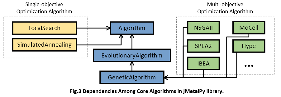
According to the source code, we find an explicit inheritance chain of each algorithm, e.g., GeneticAlgorithm -> EvolutionaryAlgorithm -> Algorithm, and NSGAII -> EvolutionaryAlgorithm -> Algorithm. In other words, jMetalPy implemented the details of specific algorithms step by step. The overall dependencies about algorithm in jMetalPy are as follows,
For better understanding the algorithm framework, I list the core part of three typical classes implemented in jMetal. Firstly, class Algorithm is the base class of all algorithms developed by jMetalPy, its run() function defines the framework of Step A,B,and C.
class Algorithm(Generic[S, R], threading.Thread, ABC)
    # core snippet of class Algorithm ...

    def run(self):
        """ Execute the algorithm. """
        self.start_computing_time = time.time()

        self.solutions = self.create_initial_solutions()  ## Step A, population initialization
        self.solutions = self.evaluate(self.solutions)    ## Step B, evaluate the 1st generation

        LOGGER.debug('Initializing progress')
        self.init_progress()

        LOGGER.debug('Running main loop until termination criteria is met')
        while not self.stopping_condition_is_met():      ## Step C, population evolution untill the stopping condition is met
            self.step()
            self.update_progress()

        self.total_computing_time = time.time() - self.start_computing_time

    # ...
Secondly, class EvolutionaryAlgorithm implements class Algorithm by completing the function step() defined in Algorithm.
class EvolutionaryAlgorithm(Algorithm[S, R], ABC):
    # core snippet of class EvolutionaryAlgorithm ...

    def step(self):
        mating_population = self.selection(self.solutions)           # Step C.1
        offspring_population = self.reproduction(mating_population)  # Step C.2
        offspring_population = self.evaluate(offspring_population)   # Step C.3
        self.solutions = self.replacement(self.solutions, offspring_population)  # Step C.4

    # ...
Thirdly, Class GeneticAlgorithm implements class EvolutionaryAlgorithm by completing detailed methods, such as reproduction() and replacement().
class GeneticAlgorithm(EvolutionaryAlgorithm[S, R]):
    # core snippet of class GeneticAlgorithm ...

    def reproduction(self, mating_population: List[S]) -> List[S]:
        number_of_parents_to_combine = self.crossover_operator.get_number_of_parents()

        if len(mating_population) % number_of_parents_to_combine != 0:
            raise Exception('Wrong number of parents')

        offspring_population = []
        for i in range(0, self.offspring_population_size, number_of_parents_to_combine):
            parents = []
            for j in range(number_of_parents_to_combine):
                parents.append(mating_population[i + j])

            offspring = self.crossover_operator.execute(parents)

            for solution in offspring:
                self.mutation_operator.execute(solution)
                offspring_population.append(solution)
                if len(offspring_population) >= self.offspring_population_size:
                    break

        return offspring_population

    def replacement(self, population: List[S], offspring_population: List[S]) -> List[S]:
        population.extend(offspring_population)
        population.sort(key=lambda s: s.objectives[0])
        return population[:self.population_size]

    def get_result(self) -> R:
        return self.solutions[0]

    # ...
In the above code snippet, there are few key points,
- the population initialization (Step A) and solution evaluation (Step B) rely on the definition of the given problem (see
jmetal.core.problem). - the crossover, mutation, and selection rely on the definition of given hyperparameters (see
jmetal.operator.crossover,jmetal.operator.mutation, andjmetal.operator.selection). - the stop criterion is usually defined by maximum loop times (see
jmetal.util.termination_criterion).
Similarly, we can also inspect the details of class NSGAII and find that the major difference between NSGAII and other algorithms is the replacement() function, where NSGAII uses a non-dominated soring and crowding distance to determine which individual should be retained.
class NSGAII(GeneticAlgorithm[S, R]):
    # core snippet of NSGAII ...

    def replacement(self, population: List[S], offspring_population: List[S]) -> List[List[S]]:
        """ This method joins the current and offspring populations to produce the population of the next generation
        by applying the ranking and crowding distance selection.
        :param population: Parent population.
        :param offspring_population: Offspring population.
        :return: New population after ranking and crowding distance selection is applied.
        """
        ranking = FastNonDominatedRanking(self.dominance_comparator)
        density_estimator = CrowdingDistance()

        r = RankingAndDensityEstimatorReplacement(ranking, density_estimator, RemovalPolicyType.ONE_SHOT)
        solutions = r.replace(population, offspring_population)

        return solutions

    def get_result(self) -> R:
        return self.solutions

    # ...
5.2 Customize our own algorithm
In jMetalPy, it's recommended to represent our algorithm as a class form, e.g., it's better to build a customized algorithm to inherit NSGAII than directly instantiate an object of NSGAII. The skeleton of a customized algorithm is like,
from jmetal.algorithm.multiobjective import NSGAII
from jmetal.operator import SBXCrossover, PolynomialMutation, BinaryTournamentSelection
from jmetal.util.termination_criterion import StoppingByEvaluations
from jmetal.util.comparator import MultiComparator
from jmetal.util.ranking import FastNonDominatedRanking
from jmetal.util.density_estimator import CrowdingDistance

class MyAlgorithm(NSGAII):

    def __init__(self, problem, population_size, offspring_population_size, mutation_ratio, crossver_ratio, max_iteration_times):
        super().__init__(problem = problem,
                         population_size = population_size,
                         offspring_population_size = offspring_population_size,
                         mutation = PolynomialMutation(probability=mutation_ratio, distribution_index=20),
                         crossover = SBXCrossover(probability=crossver_ratio, distribution_index=20),
                         selection = BinaryTournamentSelection(MultiComparator(
                                                         [FastNonDominatedRanking.get_comparator(),
                                                          CrowdingDistance.get_comparator()])),
                         termination_criterion = StoppingByEvaluations(max_evaluations=max_iteration_times)
                        )

    # def replacement(self, population, offspring_population):   # how to generate the next population

    # def reproduction(self, mating_population) # how to crossover and mutation

    # ...
Finally, we use the customized algorithm (MyAlgorithm) to solve the customized problem (MyProblem) and plot the Pareto Front.
from jmetal.util.solution import get_non_dominated_solutions
from jmetal.lab.visualization import Plot

mp = MyProblem(30)
ma = MyAlgorithm(mp, 100, 100, 1/30, 0.8, 25000)
ma.run()
front = get_non_dominated_solutions(ma.get_result())

plot_front = Plot(title='Pareto front approximation', axis_labels=['f1', 'f2'])
plot_front.plot(front, label='NSGAII-ZDT1', filename='My-ZDT1', format='png')
6. Evaluate Algorithms
Since there are many different evolutionary algorithms can be used to solve the same problem, it is imperative to compare them and choose the better ones. In single-objective algorithms, each individual has only one objective, we can simply compare the best solution found by each algorithm. While in multi-objective algorithms, things become much complicated for we need to design indicators to measure the approximation Pareto sets (i.e., non-dominated solutions) found by each algorithm. According to a prior study [1], the commonly-used indicators include Hypervolume, GD (Generational Distance), $\epsilon$, Spread, etc.
[1] Riquelme et al. "Performance metrics in multi-objective optimization." (CLEI 2015)
Here I only talk about how to use the available indicators provided by jMetal. The source code jmetal/core/quality_indicator.py has defined FitnessValue, GenerationalDistance (GD), InvertedGenerationalDistance (IGD), EpsilonIndicator ($\epsilon$), and HyperVolume.
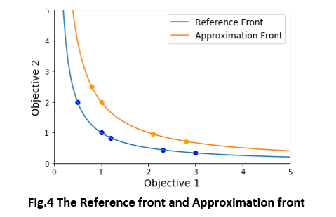
For the approximation front and reference front presented in Fig.4, here's an example of the calculation of the above indicators.
from jmetal.core.quality_indicator import GenerationalDistance,InvertedGenerationalDistance,EpsilonIndicator,HyperVolume
import numpy as np

'''
1. reference front is the ground truth for the best solution in optimization problem.
2. approximation front is the non-dominated solutions generated by algorithms.
3. reference point is used to calculated the Hypervolume, which represent the maximum value in each objective.
'''
reference_front = np.array([[0.5, 2.0], [1, 1.0], [1.2, 0.833], [2.3, 0.435], [3, 0.333]])
approximation_front = np.array([[0.8, 2.5], [1.0, 2.0], [2.1, 0.952], [2.8, 0.714]])
reference_point = [max(approximation_front[:,0]),max(approximation_front[:,0])]

'''
compute the indicators of GD, IGD, Epsilon, and Hypervolume
'''
GD = GenerationalDistance(reference_front)
print('GD:', GD.compute(approximation_front))

IGD = InvertedGenerationalDistance(reference_front)
print('IGD:', IGD.compute(approximation_front))

Epsilon = EpsilonIndicator(reference_front)
print('Epsilon:', Epsilon.compute(approximation_front))

HV = HyperVolume(reference_point)
print('Hypervolume:', HV.compute(approximation_front))